RTD (Real Time Data) is an updated alternative to DDE that allows you to dynamically link historical data to a spreadsheet.
This method offers the following advantages over DDE:
- Has Excel function-like syntax
- Can use cell references as part of the formula
- Updates in real time, frequency based on user configurations
- Is extremely efficient
USING RTD TO LINK TABULAR HISTORICAL DATA INTO EXCEL:
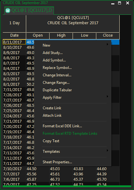
Before beginning the link, select a row to copy in the Tabular window. If you do not select a row, ProphetX will automatically copy the first row of data for you.
- Right-click and select “Format Excel RTD Template Links” from the drop-down menu
NOTE: A pop-up dialog box will display telling you that data has been copied to your computer’s internal clipboard. If you do not want to display the pop-up again, you can check-mark “Don’t display this message in the future” and it will not show again.
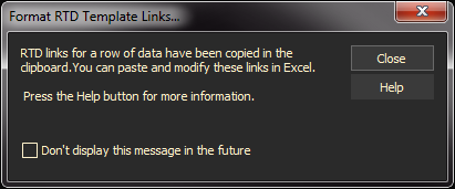
To turn it back on, go to File/Preferences or click on the Preferences check mark button on the main button bar and select Tabular. Click on Show RTD Template Message.
- To copy the link into your Excel spreadsheet, right-click a cell in Excel and select Paste.
- A single RTD link (Excel function) will be pasted into your spreadsheet. This is a “template” for you to customize and use to complete your RTD link(s).
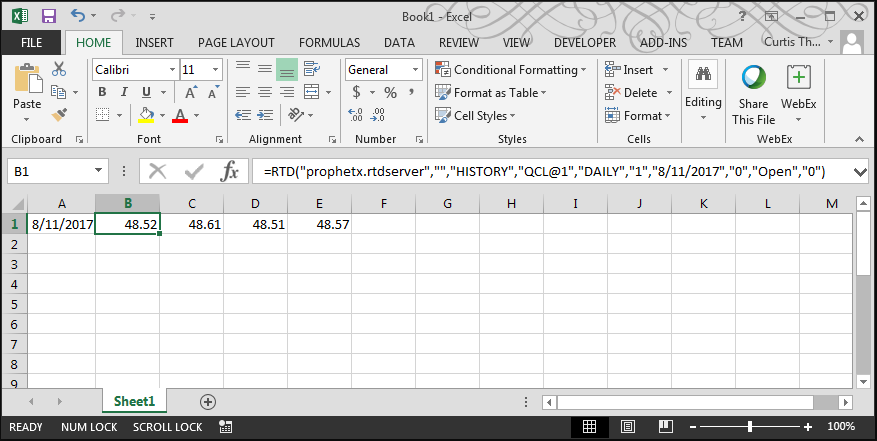
THE PROPHETX RTD FUNCTION
The ProphetX RTD Function is similar to any other Excel Function, consisting of a name, followed by a list of parameters separated by commas and enclosed in parentheses:
=RTD(“prophetx.rtdserver”,””,”RequestType”,”Symbol”,”Interval”,”Compression”,”DateTime”,”Offset”,”Field”,”BlankReplace”)
The parameters are defined as:
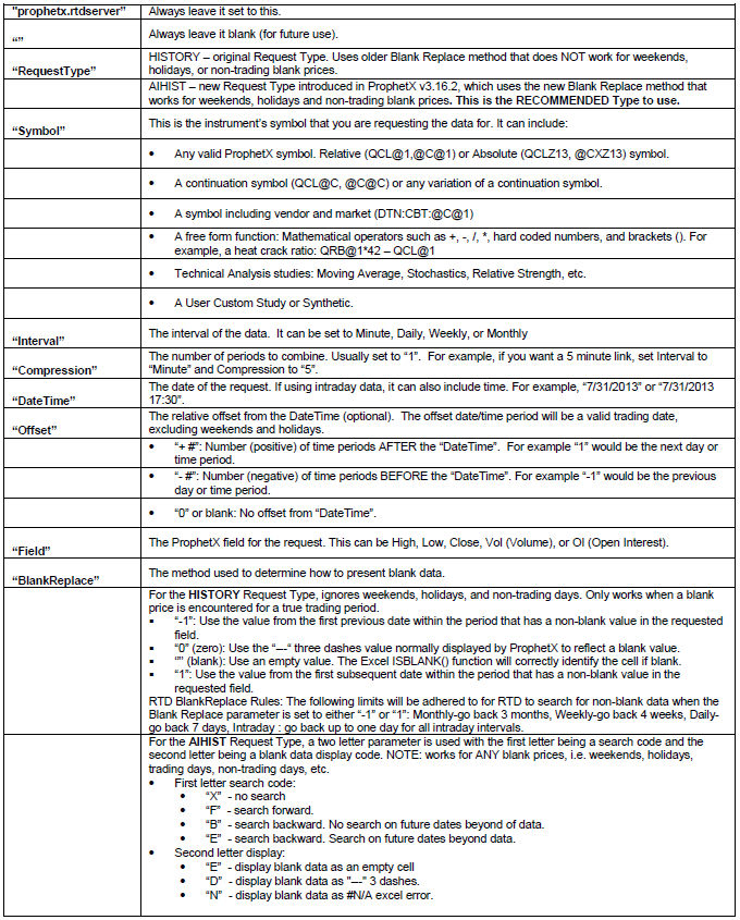
MULT Function
The MULT function is a special function created specifically for doing unit conversions on historic data that has been linked via RTD. This is automatically applied to the Excel Add-in unit conversion or can also be accomplished with a manual link.
The MULT function is used in the Symbol parameter as shown in the table above and in the Excel formula bar. It will ensure that if the underlying symbol is blank then the converted value will also be blank.
Syntax: “MULT(Symbol,Conversion Factor)” (make sure to enclose the entire formula in quotes)
Example:

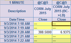
This example shows both the incremental (minute) prices for corn and the same instrument for the converted value of the underlying corn price. Notice the MULT parameter. Remember, if you use the units conversion selection in Excel Add-in this formula will be created automatically. You would manually modify the formula with the MULT parameter on data that was linked from ProphetX to your spreadsheet.
CURR Function
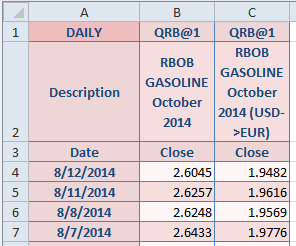
The CURR function works just like the MULT function above, but does currency conversion on historical data. This is automatically applied to the Excel Add-in currency conversion or can also be accomplished with a manual link.
The CURR function is used in the Symbol parameter as shown in the table above and in the Excel formula bar. It will ensure that if the underlying symbol is blank then the converted value will also be blank.
Syntax: “CURR(Symbol,Conversion Factor)” (make sure to enclose the entire formula in quotes)

Cell Referencing
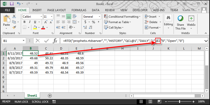
RTD Links can be modified to reference other cells in other rows and columns and copy cells the way you normally would in Excel.
For example, the link =RTD(“prophetx.rtdserver”,””,”HISTORY”,”QCL@1″,”DAILY”,”1″,”07/17/2013″,”0″,”Close”,”0″) could be changed to retrieve history from other days by changing the DateTime parameter as shown in the preceding example, to reference the date in a cell address.
Below, the RTD function in cell B3 is “referencing” the date that is in cell A3. (Notice that when you change to a cell reference you also remove the quotes (“) around the parameter.) Then the RTD function is copied into the rest of the rows in the spreadsheet (cells B4 – B8). The results show that it is retrieving the close for each date listed..
Note: In this example we manually entered the dates in the Date column. To have Excel take care of entering the dates, see additional examples below.
Cell Referencing and Replacement
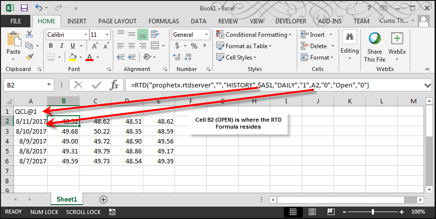
In the example below, the Symbol parameter in the RTD function in cell B3 was changed to reference the symbol in cell $A$1, telling Excel to always use that cell. Then we changed the date parameter to the cell address for the first date (A3), and copied the RTD function into the rest of the rows in the spreadsheet (cells B4 – B8). By omitting the “$’s” we are telling Excel to copy the formula and change the cell address accordingly as we copy.
Now you can enter any symbol on the fly into cell A1 and its prices will be retrieved on their corresponding dates.
Let’s look at the formula one more time. It’s telling Excel to retrieve history for the symbol in cell A1, daily, on the date referenced in cell A3 for the field CLOSE.
If we could see the formula for cell B4 if would read =RTD(“prophetx.rtdserver”,””,”HISTORY”,$A$1,”DAILY”,”1″,A4,”0″,”CLOSE”,”0″) and so on down the rows.
By duplicating/copying the RTD functions into other cells and changing the symbols, we quickly retrieved prices for additional symbols.
In the example below, QCL@1 was entered into cell D1. Cells A3 and A4 were copied in to cells D3 and D4. The date in D3 was copied down to retrieve the other date cells. Then the copied formula in cell E3 was changed to refer to the symbol in cell $D$1 and the date in cell D3. The formula was then copied in the rest of the cells in column E.
This may seem cumbersome at first, but once the formulas are set up and copied, you can now enter any symbol in cells A1 and/or cell D1 and the closes will be retrieved automatically.
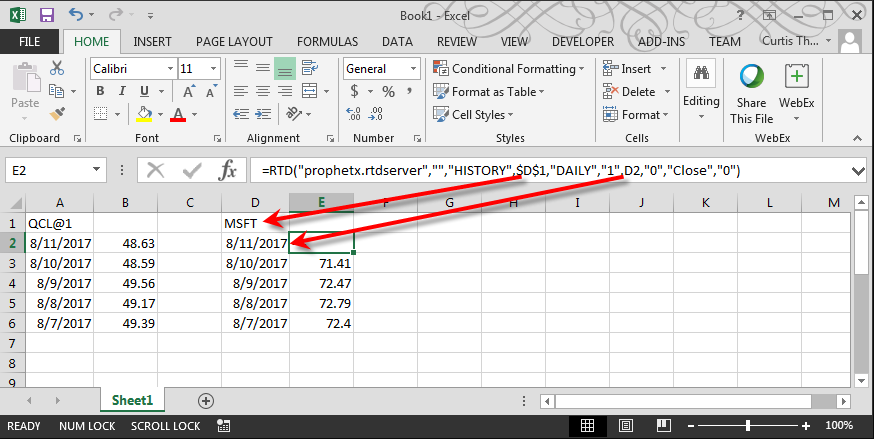
Tip: We manually entered the dates in the above examples. See next example to have Excel enter the appropriate dates.
Cell Referencing and Specific Date Range (Incremental Day)
The previous examples used static dates to retrieve the prices. But what if you want to retrieve prices for a large range of dates, but you do not want to manually enter the dates — especially when weekends and holidays are involved? There are ways to use the RTD functions and automate this process:
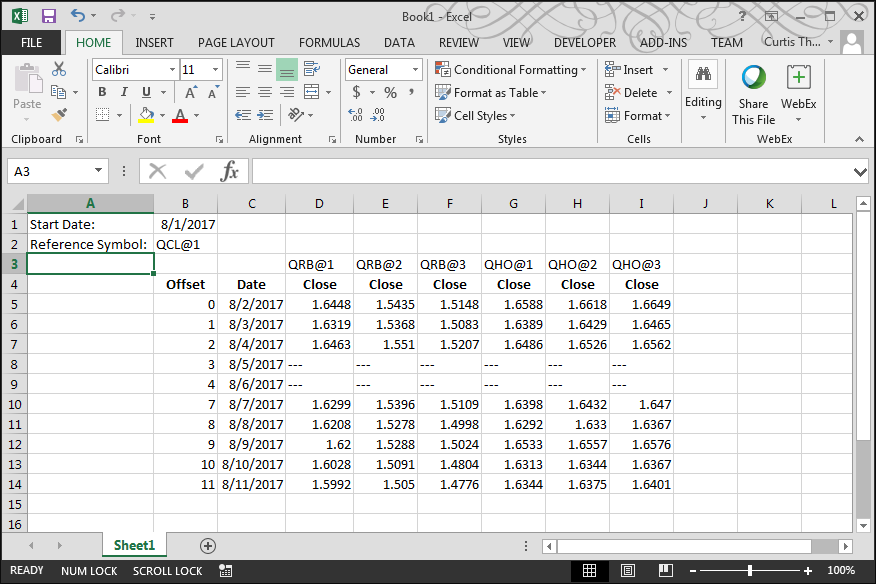
The following explains how to build the example spread displayed below:
- First, determine the exchange or market of the trading dates that you want to retrieve. For example, if you are interested in the energy market, you may want to select the NYMEX exchange. For grains, possibly the CBOT. Then select a symbol that resides in your interested exchange or market.
- Next, determine the date range for the prices you need. Basically, you need a date to start with, then will add an incremental Offset from that date.
- Start Date: we wanted prices from the start of the year (2013), so we selected “01/01/2013” as our “start date.
- Reference Symbol: we were interested in the energy market, so we selected a NYMEX symbol (QCL@1) as our “reference symbol” to represent the dates for our desired energy symbols.
- Offset: a very simple column that is numbered 0 to XX (the number of days you are interested in retrieving). Notice that you can use the special Excel feature to have it automatically create the column of numbers. Just enter a few numbers such as 0, 1, 2, 3, then highlight the cells, and grab the bottom right corner of the highlighted area and drag to create the total range of numbers.
- Date Column: this is the key RTD function that creates our specific date range. Here is the function for cell C5:
=RTD(“prophetx.rtdserver”,””,”HISTORY”,B$2,”DAILY”,”1″,B$1,B5,”Date”,”0″)
Symbol: cell B$2 which is QCL@1.
DateTime: use the Start Date, cell B$1, which is 1/1/2013.
Offset: cell B5 which is 0 days from the Start Date.
Field: retrieve the Date for the specific offset from the Start Date.
Data Retrieved: even though the Start Date is 1/1/2013, and we are using a 0 Offset, the Date retrieved is 1/2/2013, which is the first official trading day after the 1/1/2013 holiday.
Notice that each additional Date row has the identical RTD function, but the Offset references the next row. Here is cell C6
=RTD(“prophetx.rtdserver”,””,”HISTORY”,B$2,”DAILY”,”1″,B$1,B6,”Date”,”0″)
Symbol: the same as the previous RTD function
DateTime: the same as the previous RTD function
Offset: cell B6 which is 1.
Data Retrieved: the next official trading day, 1/3/2013.
- Close Column: this RTD function retrieves the Close price for the specified Date:
=RTD(“prophetx.rtdserver”,””,”HISTORY”,D$3,”DAILY”,”1″,$C5,0,”Close”,”0″)
Symbol: cell D3 which is QRB@1.
DateTime: cell $C5 which is 1/2/2013.
Offset: 0, we want the specified DateTime.
Field: retrieve the Close price.
Data Retrieved: the Close price for the referenced DateTime
Cell Referencing and Specific Date Range (Decremental Day)
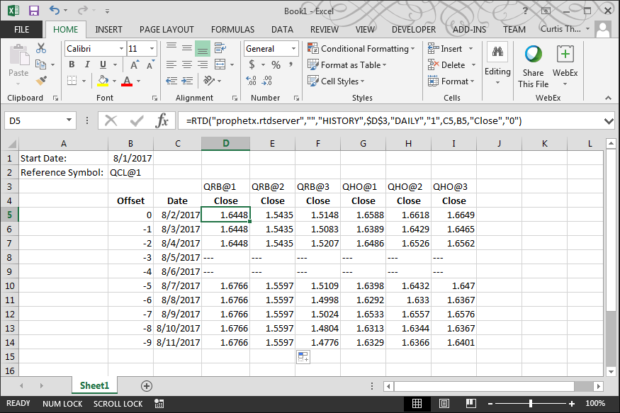
The previous example, began with a Start Date, then retrieved each subsequent date with an incrementing Offset. We could have just as easily used a decrementing Offset to retrieve each previous date. For example, if you set the DateTIme parameter to “” (blank) in the first RTD function, it will retrieve today’s date. Then set each subsequent RTD function with a decrementing Offset such as -1, -2, -3, etc. The dates retrieved would look like this:

The previous examples used Daily data. You could have also used a Weekly or Monthly interval as well.
RTD FOR INTRADAY PRICES
To use intraday data, you will have to make a few changes.
The following example can be used to retrieve minute data starting from either a specific date/time or from the current date/time.
Following, we will explain how the spreadsheet generally works, then follow with the specific contents of each cell:
Start Date and Start Time: these cells allow you to enter a specific date and time to start, or leave them blank to retrieve the most current date and time.
Interval: enter the minute interval to retrieve (1-999).
Date and Time Columns:
Row 6: the Date and Time columns for this row are the primary Date and Times used throughout the remainder of the spreadsheet. These Date and Time columns are created by referencing the Start Date and Start Time entered into cells B2 and C2, combined with the offset of 0 in cell B6.
Other Rows: the Date and Time columns for the remaining rows reference the Date and Times in Row 6 along with the associated Offset in column A
Close Columns: retrieve the Close price for the Date and Time in the associated Row.
B6: =RTD(“prophetx.rtdserver”,””,”HISTORY”,B$4,”Minute”,$C$2,$A$2+$B$2,$A6,”Date”,”0″)
C6: =RTD(“prophetx.rtdserver”,””,”HISTORY”,C$4,”Minute”,$C$2,$A$2+$B$2,$A6,”Time”,”0″)
D6: =RTD(“prophetx.rtdserver”,””,”HISTORY”,D$4,”Minute”,$C$2,$B6+$C6,,”Close”,”0″)
E6: =RTD(“prophetx.rtdserver”,””,”HISTORY”,E$4,”Minute”,$C$2,$B6+$C6,,”Close”,”0″)
F6: =RTD(“prophetx.rtdserver”,””,”HISTORY”,F$4,”Minute”,$C$2,$B6+$C6,,”Close”,”0″)
G6: =RTD(“prophetx.rtdserver”,””,”HISTORY”,G$4,”Minute”,$C$2,$B6+$C6,,”Close”,”0″)
B7: =RTD(“prophetx.rtdserver”,””,”HISTORY”,B$4,”Minute”,$C$2,$B$6+$C$6,$A7,”Date”,”0″)
C7: =RTD(“prophetx.rtdserver”,””,”HISTORY”,C$4,”Minute”,$C$2,$B$6+$C$6,$A7,”Time”,”0″)
D7: =RTD(“prophetx.rtdserver”,””,”HISTORY”,D$4,”Minute”,$C$2,$B7+$C7,,”Close”,”0″)
E7: =RTD(“prophetx.rtdserver”,””,”HISTORY”,E$4,”Minute”,$C$2,$B7+$C7,,”Close”,”0″)
F7: =RTD(“prophetx.rtdserver”,””,”HISTORY”,F$4,”Minute”,$C$2,$B7+$C7,,”Close”,”0″)
G7: =RTD(“prophetx.rtdserver”,””,”HISTORY”,G$4,”Minute”,$C$2,$B7+$C7,,”Close”,”0″)
B8: =RTD(“prophetx.rtdserver”,””,”HISTORY”,B$4,”Minute”,$C$2,$B$6+$C$6,$A8,”Date”,”0″)
C8: =RTD(“prophetx.rtdserver”,””,”HISTORY”,C$4,”Minute”,$C$2,$B$6+$C$6,$A8,”Time”,”0″)
D8: =RTD(“prophetx.rtdserver”,””,”HISTORY”,D$4,”Minute”,$C$2,$B8+$C8,,”Close”,”0″)
E8: =RTD(“prophetx.rtdserver”,””,”HISTORY”,E$4,”Minute”,$C$2,$B8+$C8,,”Close”,”0″)
F8: =RTD(“prophetx.rtdserver”,””,”HISTORY”,F$4,”Minute”,$C$2,$B9+$C9,,”Close”,”0″)
G8: =RTD(“prophetx.rtdserver”,””,”HISTORY”,G$4,”Minute”,$C$2,$B9+$C9,,”Close”,”0″)
Etc.
CELL CONCATENATION
Cell concatenation can be used in Excel to create an RTD link. Following are several examples of creating a moving average and referencing the Symbol in another cell:

B1: =RTD(“prophetx.rtdserver”,””,”HISTORY”,”MOV(QCL@1,15,0,0,0)”,”DAILY”,”1″,”8/23/2013″,”0″,”Close”,”0″)
B2: =RTD(“prophetx.rtdserver”,””,”HISTORY”,CONCATENATE(“MOV(“,A2,”,15,0,0,0)”),”DAILY”,”1″,”8/23/2013″,”0″,”Close”,”0″)
B3: =RTD(“prophetx.rtdserver”,””,”HISTORY”,”MOV(“&A3&”,15,0,0,0)”,”DAILY”,”1″,”8/23/2013″,”0″,”Close”,”0″)